 |
| 日本語 / русский / 简 体中文 / 繁 體中文 / Português / Español / Français / Nederlands / العربية |
Chapters 7 and 8 : FibrationThe mathematician Heinz Hopf describes his "fibration". Using complex numbers he builds beautiful arrangements of circles in space. |
| To Chapter 5 | To Chapter 9 |
1. Heinz Hopf and topology |
|
Topology is the science that studies deformations. For example, the cup and the tyre here on the right are of course two different objects but one can pass from one to the other by a continuous deformation that does not introduce any tear: the mathematician says that the cup and the tyre are homeomorphic (same form). And a topologist, this is somebody who can’t distinguish their cup of coffee from their donut!! There too, the theory took a very long time to achieve the status of an autonomous discipline, with its own problems and its original methods, often of a qualitative nature. Even though he had prestigious predecessors (such as Euler, Riemann, Listing or Tait), Henri Poincaré is often considered as being the one who laid the solid foundations of topology (that he called analysis situs). Our presenter, Heinz Hopf (1894-1971), is one of his most remarkable followers, in the first half of the twentieth century. |
 |
 |
|
 |
|||
 |
 |
 |
|
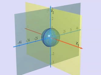
2. The sphere S3 in C2We saw that the sphere S3 of unit radius in 4 dimensional space is the set of points at distance one from the origin. If one takes four real co-ordinates x1,y1,x2,y2 in this space, the equation of this sphere is : But one can think of (x1,y1) as a complex number z1 = x1+i y1 and of (x2,y2) as a complex number z2 = x2+i y2, and the sphere S3 can then be thought as the set of pairs of complex numbers (z1,z2) such that |
|
In other words, the sphere S3 can be regarded as the unit sphere in the plane of complex dimension 2. By analogy, but only by analogy, one can thus draw the sphere S3 as a circle in a plane, but it is important not to forget that this plane is complex, that each one of its co-ordinates z1 and z2 is a complex number. The axis z2=0 for example is a complex line, therefore a real plane, and it meets the sphere S3 at the set of points (z1,0) such that |z1|2 = 1, in other words, on the circle S1. The same thing is true for the axis z1=0 but also for every line passing through the origin whose equation is of the form z2= a.z1, where a is a complex number. Thus each complex number a defines a complex line z2= a.z1 that meets the sphere S3 on a circle. There is thus a circle in S3 for each complex number a. Moreover, although the axis z1=0 is not an equation of this form, one can regard it as corresponding to a being infinite (isn’t the vertical axis a line of infinite slope?). The sphere S3 is therefore filled with circles, one for each point of S2, that is, for each complex number a (that we allow to be infinite). No two of these circles meet for different values of a. It is this decomposition of the 3 dimensional sphere into circles that one calls the Hopf fibration. |
 |
| Click the image to see a film. |
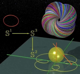 |
Recall that if X and Y are two sets, a map f from X to Y, often denoted f : X → Y, is a rule which allows us to associate to each point x of X a point f(x) in Y. For example, we can consider the Hopf map f : S3 → S2 which associates to a point (z1,z2) the point z2/z1. This deserves two explanations: First, a point of S3 is a point of the plane of complex dimension 2 and it can be described by its complex co-ordinates (z1,z2). Second, we saw, by stereographic projection, that if one adds to the plane a point at infinity, one obtains a sphere S2. And of course, the complex number z2/z1 is well defined only when z1 is nonzero and if it isn’t, we choose z2/z1 to be the point at infinity, so that z2/z1 does indeed define a point of S2. |
|
|
For each point a of S2, the set of points of S3 whose image by f is the point a (that is, the pre-image of a), which we call the fiber over a, is a circle in S3. What is the connection with the preceding explanation: quite simply that all the points of a line z2= a.z1 are such that z2/z1 is constant (obviously, because it equals a !).
|
||
3. The fibration |
|
The film first invites us to closely observe this
"fibration". For each a,
we have a circle in S3.
How do we visualize this? By stereographic projection of course! One
projects the sphere S3
onto the 3 dimensional tangent space of the pole opposite the point of
projection. This projection is a circle in space, which you can admire
(remember the lizards!). Of course, it can happen that the circle of S3
passes through the North Pole so that its stereographic projection is a
line (that is, a circle that is missing a point... that has gone to
infinity!). |
 |
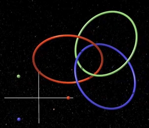 |
Several sequences illustrate the fibration : First, we see only one Hopf circle, associated with the value of a. This point a moves on the sphere S2 (remember, the complex plane plus a point at infinity) and we see that the circle moves in space and become a line from time to time, when a passes through the point at infinity. Then, we see two Hopf circles, associated with two values of a, that are both on the move. At the bottom of the screen, you see the two points a moving and simultaneously, so too do the two circles. Incidentally, notice that the two circles are linked, like two links of a chain. One cannot separate them without breaking them. Then, we see three Hopf circles for three values of a in choreographed movement ... The circles separate, approach... |
| Click the image to see a film. |
|
Finally, we see many Hopf circles at the same time. The values of a are chosen at random and the corresponding circles appear little by little. We can thus "see" that space is filled by the circles and that these circles do not meet each other. But also, we can now understand the origin of the word "fibration": all these circles are arranged like fibers of a fabric: locally, they are well organized like a packet of spaghetti. This concept of fibration, whose prototype is the Hopf map, became a central concept in topology and mathematical physics. Some fibrations are much more complicated, on spaces of much higher dimension, but it is certainly instructive to have a clear view of this historical example! To think of the real plane as a complex line is useful, but to think of the space of real dimension 4 as a plane of complex dimension 2 is even more useful! |
 |
4. The fibration ... continuedSee in the film: Chapter 8 : Fibration, continued. |
 |
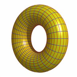
To better understand the Hopf fibration f : S3 → S2, consider a line of latitude p in S2 and then its “pre-image” p by f that is, the set of points of S3 for which the image by f is in p. Since the pre-image of each point of S2 (each fiber) is a Hopf circle and since a line of latitude is also a circle, the pre-image of p is composed of a family of circles that depends on a parameter pertaining to the circle p. So it’s a surface in S3 for which the film shows the stereographic projection in the 3 dimensional space, as usual. When a line of latitude is very close to a pole of S2 and is thus a very small circle, the pre-image of p is a small tube, in the vicinity of the fiber above this pole. When the line of latitude grows gradually, becomes the equator, then decreases again to finally approach the opposite pole, the tube grows bigger gradually then decreases again and ends up being a very fine tube. These tubes are tori in S3 but we only observe them through their projections in 3 dimensional space, so they do not appear very fine when they pass close to the North Pole of the sphere S3. |
| Click on the image to see a film. |
|
Strictly speaking, a torus is the surface of revolution in space obtained by turning a circle around an axis that is in its plane. A point of the torus has two angular co-ordinates: one to describe the position on the circle and another one to describe the angle through which the circle is turned. Notice the analogy with longitude and latitude. Beings who lived on a torus (and not on a sphere, like our Earth) would have also invented the ideas of meridian lines, parallels, longitude and latitude. |
|
In fact, the topologists often call a "torus" a surface which is "homeomorphic" to a torus of revolution, like a coffee cup for example! When they want to speak about a torus obtained by turning a circle, they make it clear by saying torus of revolution. On a torus of revolution, one clearly sees two families of circles: the meridian lines (in blue) and the parallels (in red). Distinguishing between meridian lines and parallels is now a bit more difficult. On a sphere it was easy: all the meridian lines pass through the poles, but there are no poles on a torus of revolution! One then agrees (but this is a convention only) to name the blue circles "meridians" because they lie on planes that contain the symmetry axis of the torus of revolution, and to name the red circles "parallels" because they lie on planes that are perpendicular to this axis. It is a little marvel of geometry that it is possible to trace many other circles on a torus of revolution... This chapter explains how to construct them. |
 |
|
Recall the formula which expresses the Hopf projection. In terms of the complex co-ordinates, it sends (z1,z2) to the point a considered as a point of S2. Fixing a line of latitude p in S2, is the same as fixing the modulus of a complex number, so the pre-image of a line of latitude is described by an equation of the form For example, let us choose 1 for this constant so that z1 and z2 have the same modulus. But don’t forget that so the modulus of z1 and of z2 are both equal to √2/2. Therefore, the pre-image of the line of latitude consists of the (z1,z2) where z1 and z2 are chosen arbitrarily on the circle centered at the origin with radius √2/2. Thus we see that the pre-image of the line of latitude is a surface that is parameterized by two angles : so it’s a torus, as we saw in the film. If we fix z1, we obtain a circle in S3, and if we fix z2 we obtain another circle, but for a torus of revolution in dimension 4, it is impossible to say which is a meridian and which is a parallel. When we stereographically project this torus into 3 dimensional space from the North Pole, with co-ordinates (0,1), it isn’t difficult to verify that the projection of the torus is not only homeomorphic to a torus but it is actually a torus of revolution. Revolution about which axis? Quite simply about the stereographic projection of the Hopf circle that passes through the North Pole; this projection is certainly a line! So we can see how to interpret a torus of revolution as the pre-image of a line of latitude by the Hopf map. Here is a consequence of this interpretation: for each point of the chosen line of latitude, the corresponding Hopf circle is obviously contained in the torus of revolution. We have just found other circles on the torus of revolution.... Here are some formulas. Consider the torus of
revolution in space that is obtained by projecting from the North Pole (0,1). Let's then consider the maps that send (z1,z2) to (ω.z1,z2) where ω describes the circle of complex numbers with module 1. As the modules of z1 and z2 do not change, these maps preserve the sphere S3. Points of the form (0,z2) do not change either. What we are looking at is rotations in the space of dimension 4 around the complex line z1=0. As this line passes through the projection pole (0,1), its stereographic projection is not a circle, but a straight line. Therefore, these maps that depend on the parameter ω define rotations of our space around a line. These rotations also preserve the torus of revolution that we are looking at, so that the line z1=0 is the axis of symmetry of the torus ! |
|
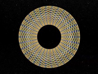
As a consequence, the parallel that passes through (z1,z2) is the set of points of the form (ω.z1, z2) where ω belongs to the circle of complex numbers of modulus 1. The meridian passing through (z1,z2) is the set of points of the form (z1, ω.z2). The Hopf circle passing through (z1,z2) is the set of points of the form (ω.z1, ω.z2) (note that if we multiply z1 and z2 by ω, we don’t change z2/z1 so all these points have the same image under f; they are in the same fiber). We don’t stop here either; through each point (z1,z2) we can also consider the "symmetric" circle of points of the form (ω.z1, ω-1.z2) which gives us a fourth circle traced on the torus of revolution. We have just shown that through each point of a torus of revolution one can draw four circles: a meridian, a parallel, a Hopf circle and the symmetric circle of a Hopf circle. |
 |
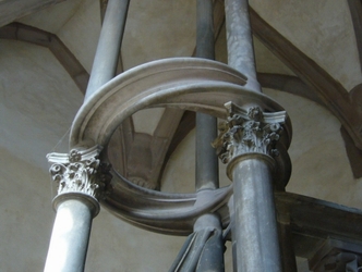 |
This fact has been known for a long time. These circles are usually called Villarceau circles, in honor of a mathematician of the nineteenth century. But, as the reader will have already realized, it is quite rare in mathematics that a theorem is due to the person whose name it carries, so long and complex is the process of creation-assimilation. Indeed, a staircase at the museum of the cathedral of Strasbourg, dating to the XVI Century shows that sculptors didn’t have to wait for Villarceau in order to cut circles on tori! |
|
The second part of this chapter depicts the Villarceau circles in a way that is independent of the Hopf fibration. Starting with a torus of revolution, one slices it by a bitangent plane and observes that the section consists of two circles. How do we prove this? One can write equations and calculate... It is possible (see here) but well, it’s not very enlightening. But algebraic geometry makes it possible to prove it in a masterful way almost without calculation, provided we use concepts such as "cyclic points". These are points that are not only infinite but also imaginary! You see, imagination is infinite! For a proof of Villarceau’s theorem with this kind of ideas, see the article. |
 |
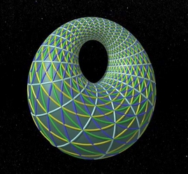 |
Given a surface in 3 dimensional space, we can regard it as a surface in S3, by adding a point at infinity. Since S3 is the unit sphere in 4 dimensional space, one can turn it by four-dimensional rotations before once more stereographically projecting it into 3 dimensional space! One obtains another surface which resembles the first but which is different! If one starts from a torus of revolution, the surfaces thus obtained are called Dupin cyclides and they were extensively studied in the nineteenth century. Since stereographic projection transforms the circles which do not pass through the pole into circles, the existence of four families of circles on the tori of revolution implies that there are also four families of circles on the cyclides... A torus in the space of dimension 3 can thus be thought of as a surface in S3 that rotates in the space of dimension 4. If we observe this through stereographic projection, we see a film where the Dupin cyclide changes shape, and at a certain moment, when the surface passes through the projection pole, becomes infinitely large, and then returns to its initial shape. However, you can see that meridians have become parallels, and vice versa, and that the torus has been turned inside out! |
| Click on the image to see a film. |
|
The geometry of the circles in space is magnificent. It sometimes bears the name of anallagmatic geometry. It is subject on which much that could be said and shown! 5. Hopf and homotopyTo finish this page, here are some brief comments on Hopf’s motivations, about which we unfortunately don’t speak in the film. In topology we often consider maps between topological spaces X and Y. We won’t give the definition here, but you can think for example that X and Y are two spheres of dimension n and p. Of course, until now we only discussed spheres of dimension 0,1,2 and 3 but you must have guessed that the story wouldn’t stop there... Of course, there isn’t much interest in studying completely arbitrary maps, and we focus on continuous maps, that is, those for which the point f(x) doesn’t change much when the change in x is sufficiently small. For example the map that associates to a real number x the number +1 if x is not zero and -1 if x is zero isn’t continuous since it "jumps" when we pass 0. But the map that associates to a number x its square x2 is continuous; if we change a number only a little, its square is only changed a little. One of the fundamental problems of topology consists of understanding continuous maps between topological spaces, such as the spheres. In fact, topology is less demanding; it seeks to understand the homotopies. Another complicated word that means something simple! Suppose that we are given two continuous maps f0 and f1 from the sphere Sn to the sphere Sp. We say that f0 and f1 are homotopic if we can deform the first one into the second. In other words, this means there is a family of maps ft that depend on a parameter t, which is a number between 0 and 1, and that connects f0 and f1. Even more precisely, this means we can associate to each x of Sn and to each number t between 0 and 1 a point ft(x) in a way that defines a continuous map of x and of t such that for t=0 we have f0 and for t=1 we have f1. |
|
For example, a map f : S1→ S2 is nothing other than a closed curve plotted on the 2 dimensional sphere. For example, the map f0 might be the one that sends all the points x of S1 to the North Pole: this is what one calls a constant map. As for the map f1, this could be for example the map that sends the circle S1 to the equator of S2. To say that these two maps are homotopic, means that we can progressively deform the equator until it becomes the North Pole. This is what you can see in the image on the right. In fact, it tuns out that this is always possible; every pair of maps S1 in S2 are always homotopic. The topologist says that all the curves plotted on the sphere S2 are homotopic to constant curves, or that S2 is simply connected. It shouldn’t be difficult either to convince yourself that the same thing is true for the spheres Sp, of all dimensions greater than or equal to two. (Check out this page too) |
|
 |
|
A map between S1 and S1 amounts transforming each point of a circle to another point on the circle: it is to some extent a curve plotted on a circle. Such a map has a degree : this is simply the number of complete revolutions that it makes. For example, the constant map does not turn at all: its degree is 0. The identity map that sends every point to itself, makes of course one revolution; its degree is 1. The map that sends any complex number of module 1 to its square doubles the argument. So as one travels once around the circle, the square makes two revolutions: its degree is 2. When a map is deformed, its degree is not changed, so there are maps of S1 to S1 that are not deformable to constant maps... It is a little more difficult to see than two maps of the same degree are deformable to each other. |
 |
But what about the maps between S2 and S2? It is similar to the case of S1 to S1; one can also define a degree, even if it is not a question any more of counting a "number of revolutions": it is now a question of counting how often the image of f "covers" the sphere and this isn’t easy to define. The simplest example is the identity: the map which sends any point to itself: its degree is 1. One may well suspect that it is not possible to deform the identity of the sphere S2 to make it constant, without tearing the sphere. But it is still necessary to prove it! The surprise came in 1931, when Heinz Hopf showed that certain maps of S3 to S2 could not be deformed continuously to constant maps. Of course, his example is the Hopf fibration which we have just met. Little by little it became an extremely important object in mathematics, but also in physics. It is the property that each pair of fibers is interlinked which underlies the fact that it is impossible to deform the Hopf map f : S3→ S2 to a constant map. It would require a lengthy explanation to give a convincing justification! See this book for a complete but difficult exposition or even Hopf’s original article for a proof and many more details. |
|
What does one know about the maps between Sn and Sp with arbitrary values of n and p? Many things are known, but we are far from knowing everything: the "homotopy classes of the maps between spheres" remain largely a mystery! The "Hopf fibration" is only one of the contributions of Heinz Hopf. He had a profound impact on the mathematics of the twentieth century. |
| To chapter 5 | To chapter 9 |